Thermophysical Property Database
This database contains data on density, surface tension and viscosity coefficient of metals, alloys and ceramics obtained by floating experiments using an electrostatic levitation furnace.
The electrostatic floating method utilizes the Coulomb force acting between the charged sample and the electrode placed around it.Since it does not require a container to hold the molten liquid, mixing of impurities is prevented and accurate measurement is enabled.
This database was constructed in a JAXA-NIMS collaboration framework on materials property data utilization for academic and industrial applications (started from August 1st, 2017).
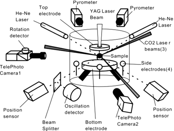
Electrostatic levitation furnace
For New Users
To use MatNavi, "DICE Account User Registration", "Domain Name Registration of E-mail Address", and "MatNavi Usage Application" are required. Please see the link for details.
Mass downloading of data is prohibited
Web scraping of data is prohibited!
The acquisition of large amounts of data, whether by manual or mechanical means, is prohibited by the MatNavi Service Terms of Use.
User accounts will be suspended when there is a possibility of data access that is deemed to be a violation.
Please comply with the terms of use, as the MatNavi database service will no longer be viable.
Number of open data
| Number of experiments | Density measurement experiment | 162 |
|---|---|---|
| Drop vibration experiment | 106 | |
| Number of characteristic data | Density | 176 |
| Surface tension | 99 | |
| Viscosity coefficient | 110 | |
| The number of samples | Pure metal | 91 |
| Alloy | 124 | |
| Ceramics | 53 |
Experiment overview
|
■ Density acquisition experiment
Start
 
① Standard sample calibration experiment
② Still image segmentation 1
③ Image analysis 1
④ density measurement experiment
⑤ sample heating / quenching
⑥ Correction of melting point
⑦ Still image segmentation 2
⑧ Image analysis 2
⑨ Volume calculation
⑩ Mass measurement
⑪ Density calculation
⑫ Equation of temperature compensation formula
⑬ Equation of density-temperature relational expression
End
|
① Standard samples (such as stainless steel) are floated and calibrated using an electrostatic levitation furnace. ② Cut out still images for image analysis from the movie data recorded in ①. ③ Analyze the image file cut out in ② and calculate the number of pixels Pixel / mm (H), Pixel / mm (V) for camera calibration.For the analysis of the image, fitting of the contour is performed by using the harmonic function represented by the following Lucian dollar polynomial Pn(cos θ). ④ Suspend the sample. ⑤ Heat with reference to the melting point of the sample. ⑥ Correct the temperature measured in ⑤ with the melting point temperature during rapid cooling. ⑦ Cut out a still image for image analysis from the movie data recorded in ⑤Synchronize the cutout time with the temperature data. ⑧ Analysis of the image file cut out in ⑦ and fitting of contour The model formula is the same as ③ image analysis. The data output in the image analysis are fitting coefficients B0 to B5, sample center position x, y , And the value Rss of the error function. ⑨ The volume is calculated from the calculated R(θ). ⑩ The sample is collected and the mass is measured. ⑪ Density is calculated from the calculated volume and mass. ⑫ Make a regression equation based on the temperature data corrected by the temperature melting point during quenching. ⑬ An approximate expression of the density-temperature relation is made using the calculated density and temperature data. |
|
■Droplet vibration experiment
Start
① Surface tension / viscosity coefficient Measurement experiment
② Droplet vibration experiment
③ Still image segmentation 3
④ Image analysis 3
⑤ sample radius / flatness ratio calculated
⑥ Simple analysis
⑦ Nonlinear Fitting
⑧ Identification of sample rotation speed
⑨ Correction of rotation
⑩ Correction of charge / gravity
⑪ Surface tension calculation
⑫ Calculation of viscosity coefficient
End
|
① Suspend the sample. ② Apply voltage to excite droplet vibration The excited vibration is the second order vibration mode as shown below, then cut off and attenuate the voltage. 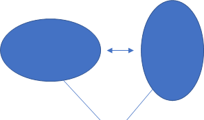 sample ③ Choose beautiful waveform data from the sample movie data when droplet vibration of ② and extract the still image. ④ Analyze the sample image The procedure is the same as ③ in Density experiment. Calculate shape approximation coefficient, pixel number dh, dv. ⑤ Calculate sample radius and oblateness from the result of ⑤. ⑥ Calculate the resonance frequency ω and the damping coefficient τ using the vibration data and the model equation by simple analysis When the shape of the sample undergoes minute deformation of the axis target as shown in the above figure, the time change r(t) Is described as follows. r 0 is the sample diameter at the time of spherical formation and is calculated by ⑤.P n (cosθ) is an nth order Lucian polynomial, θ is the angle between the z axis direction and the radial direction, and r n is the amplitude according to the n th order vibration mode.At this time, the resonance frequency ω n and the resonance coefficient τ n are expressed as follows using the expression of Rayleigh * . σ is the surface tension of the droplet, p is the density, and η is the viscosity coefficient.Here, substituting n = 2 in this experiment gives the resonance frequency ω 2 and the damping coefficient τ 2 as follows. ⑦ Fitting is performed to increase the frequency when the amplitude of the droplet is large by FFT analysis using the result obtained by the simple analysis of ⑥. In the above equation, A represents the amplitude and Φ represents the phase shift, and the resonance frequency ω 2 is as follows. ⑧ In order to correct the influence of the rotation of the sample, frequency shift ⊿ω (%) and damping coefficient shift ⊿τ (%) is calculated from the flattening ratio. ⑨ Calculate 2.23 * τ as the time when the attenuation is the first 1/10, and calculate the final ω and τ using ⊿ω and ⊿τ calculated in ⑧. ⑩ Correct errors due to surface charge and gravity effects.Charge correction by Rayleigh * model is given by the following equation. 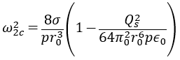 In addition, the correction of gravity is as follows.Q s is a charge, and ε 0 is a vacuum dielectric constant. ⑪ Calculate the viscosity coefficient from sample radius, density, τ. ⑫ Surface tension is calculated from sample radius, density, ω. |
Link to JAXA Related
Citing the database
Please cite Thermophysical Property using the database URL.
●Database URL
Thermophysical Property Database: https://thermophys.nims.go.jp/ National Institute for Materials Science (NIMS), accessed {date-of-your-access}.
Related: How to mention our service in acknowledgments
Disclaimer
- National Institute for Materials Science (NIMS) holds the copyright of this database system.
- No reproduction, republication or distribution to third parties of any content is permitted without written permission of NIMS.
- NIMS takes no responsibility for any damage incurred by the user as a result of using this database system.
System Requirements
Browser : Microsoft Edge, Google Chrome, Firefox